SIR-X
This notebook exemplifies how Open-SIR can be used to fit the SIR-X model by Maier and Dirk (2020) to existing data and make predictions. The SIR-X model is a standard generalization of the Susceptible-Infectious-Removed (SIR) model, which includes the influence of exogenous factors such as policy changes, lockdown of the whole population and quarantine of the infectious individuals.
The Open-SIR implementation of the SIR-X model will be validated reproducing the parameter fitting published in the supplementary material of the original article published by Maier and Brockmann (2020). For simplicity, the validation will be performed only for the city of Guangdong, China.
Import modules
[1]:
# Uncomment this cell to activate black code formatter in the notebook
# %load_ext nb_black
[2]:
# Import packages
import pandas as pd
import matplotlib.pyplot as plt
import numpy as np

%matplotlib inline
Data sourcing
We will source data from the repository of the [John Hopkins University COVID-19 dashboard] (https://coronavirus.jhu.edu/map.html) published formally as a correspondence in The Lancet. This time series data contains the number of reported cases \(C(t)\) per day for a number of cities.
[3]:
# Source data from John Hokpins university reposotiry
# jhu_link = "https://raw.githubusercontent.com/CSSEGISandData/COVID-19/master/who_covid_19_situation_reports/who_covid_19_sit_rep_time_series/who_covid_19_sit_rep_time_series.csv"
jhu_link = "https://raw.githubusercontent.com/CSSEGISandData/COVID-19/master/csse_covid_19_data/csse_covid_19_time_series/time_series_covid19_confirmed_global.csv"
jhu_df = pd.read_csv(jhu_link)
# Explore the dataset
jhu_df.head(10)
[3]:
| Province/State | Country/Region | Lat | Long | 1/22/20 | 1/23/20 | 1/24/20 | 1/25/20 | 1/26/20 | 1/27/20 | ... | 7/2/20 | 7/3/20 | 7/4/20 | 7/5/20 | 7/6/20 | 7/7/20 | 7/8/20 | 7/9/20 | 7/10/20 | 7/11/20 | |
|---|---|---|---|---|---|---|---|---|---|---|---|---|---|---|---|---|---|---|---|---|---|
| 0 | NaN | Afghanistan | 33.0000 | 65.0000 | 0 | 0 | 0 | 0 | 0 | 0 | ... | 32022 | 32324 | 32672 | 32951 | 33190 | 33384 | 33594 | 33908 | 34194 | 34366 |
| 1 | NaN | Albania | 41.1533 | 20.1683 | 0 | 0 | 0 | 0 | 0 | 0 | ... | 2662 | 2752 | 2819 | 2893 | 2964 | 3038 | 3106 | 3188 | 3278 | 3371 |
| 2 | NaN | Algeria | 28.0339 | 1.6596 | 0 | 0 | 0 | 0 | 0 | 0 | ... | 14657 | 15070 | 15500 | 15941 | 16404 | 16879 | 17348 | 17808 | 18242 | 18712 |
| 3 | NaN | Andorra | 42.5063 | 1.5218 | 0 | 0 | 0 | 0 | 0 | 0 | ... | 855 | 855 | 855 | 855 | 855 | 855 | 855 | 855 | 855 | 855 |
| 4 | NaN | Angola | -11.2027 | 17.8739 | 0 | 0 | 0 | 0 | 0 | 0 | ... | 315 | 328 | 346 | 346 | 346 | 386 | 386 | 396 | 458 | 462 |
| 5 | NaN | Antigua and Barbuda | 17.0608 | -61.7964 | 0 | 0 | 0 | 0 | 0 | 0 | ... | 69 | 68 | 68 | 68 | 70 | 70 | 70 | 73 | 74 | 74 |
| 6 | NaN | Argentina | -38.4161 | -63.6167 | 0 | 0 | 0 | 0 | 0 | 0 | ... | 69941 | 72786 | 75376 | 77815 | 80447 | 83426 | 87030 | 90693 | 94060 | 97509 |
| 7 | NaN | Armenia | 40.0691 | 45.0382 | 0 | 0 | 0 | 0 | 0 | 0 | ... | 26658 | 27320 | 27900 | 28606 | 28936 | 29285 | 29820 | 30346 | 30903 | 31392 |
| 8 | Australian Capital Territory | Australia | -35.4735 | 149.0124 | 0 | 0 | 0 | 0 | 0 | 0 | ... | 108 | 108 | 108 | 108 | 108 | 111 | 112 | 113 | 113 | 113 |
| 9 | New South Wales | Australia | -33.8688 | 151.2093 | 0 | 0 | 0 | 0 | 3 | 4 | ... | 3211 | 3405 | 3419 | 3429 | 3433 | 3440 | 3453 | 3467 | 3474 | 3478 |
10 rows × 176 columns
It is observed that the column “Province/States” contains the name of the cities, and since the forth column a time series stamp (or index) is provided to record daily data of reported cases. Additionally, there are many days without recorded data for a number of chinese cities. This won’t be an issue for parameter fitting as Open-SIR doesn’t require uniform spacement of the observed data.
Data preparation
In the following lines, the time series for Guangdong reported cases \(C(t)\) is extracted from the original dataframe. Thereafter, the columns are converted to a pandas date time index in order to perform further data preparation steps.
[4]:
China = jhu_df[jhu_df[jhu_df.columns[1]] == "China"]
city_name = "Guangdong"
city = China[China["Province/State"] == city_name]
city = city.drop(columns=["Province/State", "Country/Region", "Lat", "Long"])
time_index = pd.to_datetime(city.columns)
data = city.values
# Visualize the time
ts = pd.Series(data=city.values[0], index=time_index)
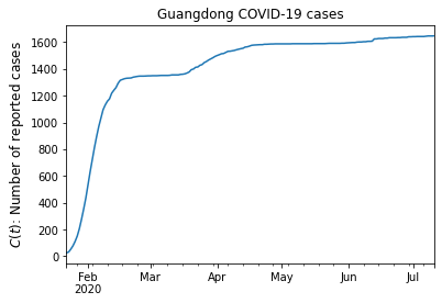
Using the function ts.plot() a quick visualization of the dataset is obtained:
[5]:
ts.plot()
plt.title("Guangdong COVID-19 cases")
plt.ylabel("$C(t)$: Number of reported cases", size=12)
plt.show()
Data cleaning
[6]:
ts_clean = ts.dropna()
# Extract data
ts_fit = ts_clean["2020-01-21":"2020-02-12"]
# Convert index to numeric
ts_num = pd.to_numeric(ts_fit.index)
t0 = ts_num[0]
# Convert datetime to days
t_days = (ts_num - t0) / (10 ** 9 * 86400)
t_days = t_days.astype(int).values
# t_days is an input for SIR
[7]:
# Define the X number
nX = ts_fit.values  # Number of infected
N = 104.3e6  # Population size of Guangdong
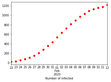
Exploration of the dataset
[8]:
ts_fit.plot(style="ro")
plt.xlabel("Number of infected")
plt.show()
[ ]:
Setting up SIR and SIR-X models
The population \(N\) of the city is a necessary input for the model. In this notebook, this was hardocded, but it can be sourced directly from a web source.
Note that whilst the SIR model estimates directly the number of infected people, \(N I(t)\), SIR-X estimates the number of infected people based on the number of tested cases that are in quarantine or in an hospital \(N X(t)\)
[9]:
# These lines are required only if opensir wasn't installed using pip install, or if opensir is running in the pipenv virtual environment
import sys

path_opensir = "../../"
sys.path.append(path_opensir)

# Import SIR and SIRX models
from opensir.models import SIR, SIRX

nX = ts_fit.values  # Number of observed infections of the time series
N = 104.3e6  # Population size of Guangdong
params = [0.95, 0.38]
w0 = (N - nX[0], nX[0], 0)

G_sir = SIR()
G_sir.set_params(p=params, initial_conds=w0)
G_sir.fit_input = 2
G_sir.fit(t_days, nX)
G_sir.solve(t_days[-1], t_days[-1] + 1)
t_SIR = G_sir.fetch()[:, 0]
I_SIR = G_sir.fetch()[:, 2]
Try to fit a SIR model to Guangdong data
[10]:
ax = plt.axes()
ax.tick_params(axis="both", which="major", labelsize=14)
plt.plot(t_SIR, I_SIR)
plt.plot(t_days, nX, "ro")
plt.show()
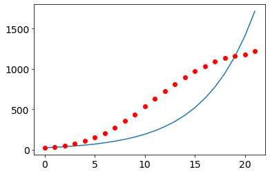
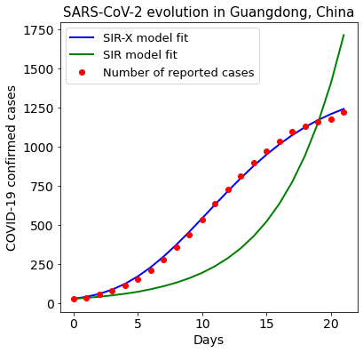
The SIR model is clearly not appropriate to fit this data, as it cannot resolve the effect of exogeneous containment efforts such as quarantines or lockdown. We will repeat the process with a SIR-X model.
Fit SIR-X to Guangdong Data
[11]:
g_sirx = SIRX()
params = [6.2 / 8, 1 / 8, 0.05, 0.05, 5]
# X_0 can be directly ontained from the statistics
n_x0 = nX[0]  # Number of people tested positive
n_i0 = nX[0]

w0 = (N - n_x0 - n_i0, n_i0, 0, n_x0)
g_sirx.set_params(p=params, initial_conds=w0)
# Fit all parameters
fit_index = [False, False, True, True, True]
g_sirx.fit(t_days, nX, fit_index=fit_index)
g_sirx.solve(t_days[-1], t_days[-1] + 1)
t_sirx = g_sirx.fetch()[:, 0]
inf_sirx = g_sirx.fetch()[:, 4]
[12]:
plt.figure(figsize=[6, 6])
ax = plt.axes()
plt.plot(t_sirx, inf_sirx, "b-", linewidth=2)
plt.plot(t_SIR, I_SIR, "g-", linewidth=2)
plt.plot(t_days, nX, "ro")
plt.legend(
    ["SIR-X model fit", "SIR model fit", "Number of reported cases"], fontsize=13
)
plt.title("SARS-CoV-2 evolution in Guangdong, China", size=15)
plt.xlabel("Days", fontsize=14)
plt.ylabel("COVID-19 confirmed cases", fontsize=14)
ax.tick_params(axis="both", which="major", labelsize=14)
plt.show()
After fitting the parameters, the effective infectious period \(T_{I,eff}\) and the effective reproduction rate \(R_{0,eff}\) can be obtained from the model properties
Aditionally, the Public containment leverage \(P\) and the quarantine probability \(Q\) can be calculated through:
[13]:
print("Effective infectious period T_I_eff =  %.2f days " % g_sirx.t_inf_eff)
print(
    "Effective reproduction rate R_0_eff =  %.2f, Maier and Brockmann = %.2f"
    % (g_sirx.r0_eff, 3.02)
)
print(
    "Public containment leverage =  %.2f, Maier and Brockmann = %.2f"
    % (g_sirx.pcl, 0.75)
)
print(
    "Quarantine probability =  %.2f, Maier and Brockmann = %.2f" % (g_sirx.q_prob, 0.51)
)
Effective infectious period T_I_eff =  3.89 days
Effective reproduction rate R_0_eff =  3.01, Maier and Brockmann = 3.02
Public containment leverage =  0.80, Maier and Brockmann = 0.75
Quarantine probability =  0.51, Maier and Brockmann = 0.51
Make predictions using model.predict
[14]:
# Make predictions and visualize
# Obtain the results 14 days after the train data ends
sirx_pred = g_sirx.predict(14)
print("T n_S \t   n_I \tn_R \tn_X")
for i in sirx_pred:
    print(*i.astype(int))
T n_S      n_I  n_R     n_X
0 11450984 227 92847569 1219
1 10307571 190 93990991 1246
2 9278326 158 95020245 1269
3 8351856 130 95946723 1288
4 7517894 107 96780694 1304
5 6767209 87 97531385 1317
6 6091483 70 98207117 1327
7 5483230 57 98815376 1336
8 4935707 45 99362903 1342
9 4442871 36 99855743 1348
10 3999251 29 100299366 1352
11 3599916 23 100698704 1356
12 3240456 18 101058166 1358
13 2916888 14 101381735 1361
14 2625630 11 101672995 1362
Prepare date time index to plot predictions
[15]:
# Import datetime module from the standard library
import datetime

# Obtain the last day from the data used to train the model
last_time = ts_fit.index[-1]
# Create a date time range based on the number of rows of the prediction
numdays = sirx_pred.shape[0]
day_zero = datetime.datetime(last_time.year, last_time.month, last_time.day)
date_list = [day_zero + datetime.timedelta(days=x) for x in range(numdays)]
Plot predictions
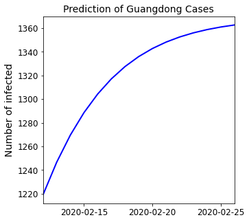
[16]:
# Extract figure and axes
fig, ax = plt.subplots(figsize=[5, 5])
# Create core plot attributes
plt.plot(date_list, sirx_pred[:, 4], color="blue", linewidth=2)
plt.title("Prediction of Guangdong Cases", size=14)
plt.ylabel("Number of infected", size=14)
# Remove trailing space
plt.xlim(date_list[0], date_list[-1])
# Limit the amount of data displayed
ax.xaxis.set_major_locator(plt.MaxNLocator(3))
# Increase the size of the ticks
ax.tick_params(labelsize=12)
plt.show()
Calculation of predictive confidence intervals
The confidence intervals on the predictions of the SIR-X model can be calculated using a block cross validation. This technique is widely used in Time Series Analysis. In the open-sir API, the function model.ci_block_cv calculates the average mean squared error of the predictions, a list of the rolling mean squared errors and the list of parameters which shows how much each parameter changes taking different number of days for making predictions.
The three first parameters are the same as the fit function, while the last two parameters are the lags and the min_sample. The lags parameter indicates how many periods in the future will be forecasted in order to calculate the mean squared error of the model prediction. The min_sample parameter indicates the initial number of observations and days that will be taken to perform the block cross validation.
In the following example, model.ci_block_cv is used to estimate the average mean squared error of 1-day predictions taking 6 observations as the starting point of the cross validation. For Guangdong, a min_sample=6 higher than the default 3 is required to handle well the missing data. This way, both the data on the four first days, and two days after the data starts again, are considered for cross validation.
[17]:
# Calculate confidence intervals
mse_avg, mse_list, p_list, pred_data = g_sirx.block_cv(lags=1, min_sample=6)
If it is assumed that the residuals distribute normally, then a good estimation of a 95% confidence interval on the one-day prediction of the number of confirmed cases is
Where \(n_{X,{t+1}}\) is the real number of confirmed cases in the next day, and \(\hat{n}_{X,{t+1}}\) is the estimation using the SIR-X model using cross validation. We can use the PredictionResults instance pred_data functionality to explore the mean-squared errors and the predictions confidence intervals:
[18]:
pred_data.print_mse()
Average MSE for 0-day predictions = 18.16, MSE sample size = 16
Average MSE for 1-day predictions = 28.81, MSE sample size = 15
Average MSE for 2-day predictions = 40.23, MSE sample size = 14
Average MSE for 3-day predictions = 54.97, MSE sample size = 13
Average MSE for 4-day predictions = 73.92, MSE sample size = 12
Average MSE for 5-day predictions = 95.56, MSE sample size = 11
Average MSE for 6-day predictions = 119.34, MSE sample size = 10
Average MSE for 7-day predictions = 145.10, MSE sample size = 9
Average MSE for 8-day predictions = 172.19, MSE sample size = 8
Average MSE for 9-day predictions = 198.89, MSE sample size = 7
Average MSE for 10-day predictions = 223.80, MSE sample size = 6
Average MSE for 11-day predictions = 245.12, MSE sample size = 5
Average MSE for 12-day predictions = 283.18, MSE sample size = 4
Average MSE for 13-day predictions = 266.35, MSE sample size = 3
Average MSE for 14-day predictions = 92.48, MSE sample size = 2
Average MSE for 15-day predictions = 196.84, MSE sample size = 1
The predictive accuracy of the model is quite impressive, even for 9-day predictions. Let’s take advantage of the relatively low mean squared error to forecast a 10 days horizon with confidence intervals using pred_data.plot_predictions(n_days=9)
[19]:
pred_data.plot_pred_ci(n_days=9)
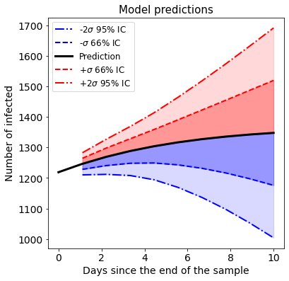
If it is assumed that the residuals distribute normally, then a good estimation of a 95% confidence interval on the one-day prediction of the number of confirmed cases is
Where \(n_{X,{t+1}}\) is the real number of confirmed cases in the next day, and \(\hat{n}_{X,{t+1}}\) is the estimation using the SIR-X model using cross validation. We use solve to make a 1-day prediction and append the 95% confidence interval.
[20]:
# Predict
g_sirx.solve(t_days[-1] + 1, t_days[-1] + 2)
n_X_tplusone = g_sirx.fetch()[-1, 4]
print("Estimation of n_X_{t+1} = %.0f +- %.0f " % (n_X_tplusone, 2 * mse_avg[0]))
Estimation of n_X_{t+1} = 1268 +- 36
[21]:
# Transform parameter list into a DataFrame
par_block_cv = pd.DataFrame(p_list)
# Rename dataframe columns based on SIR-X parameter names
par_block_cv.columns = g_sirx.PARAMS
# Add the day. Note that we take the days from min_sample until the end of the array, as days
# 0,1,2 are used for the first sampling in the block cross-validation
par_block_cv["Day"] = t_days[5:]
# Explore formatted dataframe for parametric analysis
par_block_cv.head(len(p_list))
[21]:
| alpha | beta | kappa_0 | kappa | inf_over_test | Day | |
|---|---|---|---|---|---|---|
| 0 | 0.775 | 0.125 | 0.115899 | 1.020877e-10 | 2.705780 | 5 |
| 1 | 0.775 | 0.125 | 0.109540 | 4.023231e-13 | 2.774667 | 6 |
| 2 | 0.775 | 0.125 | 0.068467 | 1.099828e-01 | 1.818714 | 7 |
| 3 | 0.775 | 0.125 | 0.082939 | 6.627930e-02 | 2.100077 | 8 |
| 4 | 0.775 | 0.125 | 0.104995 | 6.901938e-11 | 2.822296 | 9 |
| 5 | 0.775 | 0.125 | 0.090598 | 4.458775e-02 | 2.285169 | 10 |
| 6 | 0.775 | 0.125 | 0.092793 | 3.733649e-02 | 2.355333 | 11 |
| 7 | 0.775 | 0.125 | 0.104239 | 1.903129e-09 | 2.824648 | 12 |
| 8 | 0.775 | 0.125 | 0.105289 | 3.024668e-09 | 2.843301 | 13 |
| 9 | 0.775 | 0.125 | 0.106338 | 7.624121e-11 | 2.866025 | 14 |
| 10 | 0.775 | 0.125 | 0.107283 | 1.264505e-10 | 2.889912 | 15 |
| 11 | 0.775 | 0.125 | 0.108250 | 3.590963e-14 | 2.917548 | 16 |
| 12 | 0.775 | 0.125 | 0.108956 | 1.935729e-15 | 2.939909 | 17 |
| 13 | 0.775 | 0.125 | 0.110043 | 8.197801e-11 | 2.977366 | 18 |
| 14 | 0.775 | 0.125 | 0.109884 | 4.608366e-03 | 2.954701 | 19 |
| 15 | 0.775 | 0.125 | 0.106441 | 2.069015e-02 | 2.797521 | 20 |
| 16 | 0.775 | 0.125 | 0.104914 | 2.805141e-02 | 2.739572 | 21 |
[22]:
plt.figure(figsize=[5, 5])
ax = plt.axes()
ax.tick_params(axis="both", which="major", labelsize=14)
plt.plot(mse_list[0], "ro")
plt.xlabel("Number of days used to predict the next day", size=14)
plt.ylabel("MSE", size=14)
plt.show()
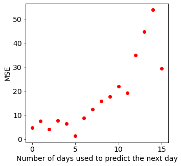
There is an outlier on day 1, as this is when the missing date starts. A more reliable approach would be to take the last 8 values of the mean squared error to calculate a new average assuming that there will be no more missing data.
Variation of fitted parameters
Finally, it is possible to observe how the model parameters change as more days and number of confirmed cases are introduced in the block cross validation.
It is clear to observe that after day 15 all parameters except kappa begin to converge. Therefore, care must be taken when performing inference over the parameter kappa.
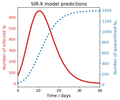
Long term prediction
Now we can use the model to predict when the peak will occur and what will be the maximum number of infected
[23]:
# Predict
plt.figure(figsize=[6, 6])
ax = plt.axes()
ax.tick_params(axis="both", which="major", labelsize=14)
g_sirx.solve(40, 41)
# Plot
plt.plot(g_sirx.fetch()[:, 4], "b-", linewidth=2)  # X(t)
plt.plot(g_sirx.fetch()[:, 2], "b--", linewidth=2)  # I(t)
plt.xlabel("Day", size=14)
plt.ylabel("Number of people", size=14)
plt.legend(["X(t): Confirmed", "I(t) = Infected"], fontsize=13)
plt.title(city_name)
plt.show()
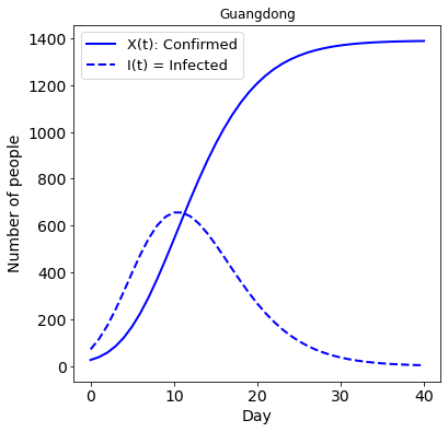
The model was trained with a limited amount of data. It is clear to observe that since the measures took place in Guangdong, at least 6 weeks of quarantine were necessary to control the pandemics. Note that a limitation of this model is that it predicts an equilibrium where the number of infected, denoted by the yellow line in the figure above, is 0 after a short time. In reality, this amount will decrease to a small number.
After the peak of infections is reached, it is necessary to keep the quarantine and effective contact tracing for at least 30 days more.
Validate long term plot using model.plot()
The function model.plot() offers a handy way to visualize model fitting and predictions. Custom visualizations can be validated against the model.plot() function.
[24]:
g_sirx.plot()